Anomalies Detection in Time Series

The number of devices, systems, services and platforms belonging to industrial, informational and cyber-physical spheres arоund us increases daily. Usually, we do not bother thinking about how a coffee machine makes a cup of coffee, how a robot vacuum cleaner determines the best cleaning routes, how a biometric identification system identifies people on a video or government services portal processes our requests. Everyone got used to these systems, considering them “black boxes” with predictable outputs, and never accounting for these systems’ health. While this is excusable and even expectable for a user, developing companies and those who implement technological systems in their work should have a different point of view. This article covers one of the methods of anomalies detection in time series, namely states, which can help determine if a system is “struggling” (or is about to struggle).

An efficient operation of a complicated technological system requires various analytics and monitoring methods ensuring control, management, and proactive modification of different parameters. Typically, monitoring is executed via different common tools (such as reliable event collection and visualization systems). On the other hand, creating efficacious analytic tools requires additional research, experiments, and excellent knowledge of the subject area. Data analysis methods can be divided into four basic types [1]:

• descriptive analytics visualizes the accumulated data, including transformed and interpreted data in order to provide a view of the entire picture. While it is the simplest type of analysis, it is also the most important type for other analysis methods application;
• diagnostic analytics is aimed at finding the causes of the events that had taken place in the past and at the same time at identifying trends, anomalies, and characteristic features of the described process, its cause, and correlations (interrelations);
• predictive analytics creates a forecast based on the identified trends and statistical models derived from historical data;
• prescriptive analytics recommends the best solution for the task based on predictive analytics, for instance, recommendations on equipment operation and business processes optimization or a list of measures preventing emergency conditions.

Predictive and prescriptive analytic often relies on modeling methods including machine learning. The model effectiveness level depends on the quality of data collection, processing, and preliminary analysis. The forementioned types of analytics differ by the complexity of applied models and by the required degree of human intervention.

There are a lot of spheres where analytics tools can be implemented: information security, banking, public administration, medicine, etc. The same method is often effective for different subject areas. Therefore, analytics system developers tend to create universal modules, containing various algorithms.

Most technological system monitoring results can be represented as time series [2]. The most important properties of a time-series are:

• binding each measurement (sample, discrete) to the time of its appearance;
• equal time-distance between measurements;
• possibility to reconstruct process behavior in current and future periods based on the data obtained in the previous periods.

Fig. 1. Time series

Time series capabilities are not limited to numerically measured process descriptions. Using various methods and model architectures, including deep learning neural networks, allows working with data related to natural language processing (NLP), computer vision (CV), etc. For example, chat messages can be converted to numeric vectors (embeddings) sequentially appearing at a certain time, and video is nothing more than a time-dependent numeric matrix.

Time series are handy for describing complex devices operation and are often applied in typical tasks such as modeling, prediction, feature selection, classification, clusterization, pattern recognition, anomalies detection. Use examples include electrocardiogram tracing, change of stocks’ and currencies’ prices, weather forecast value, network traffic volume, engine operation parameters, etc.

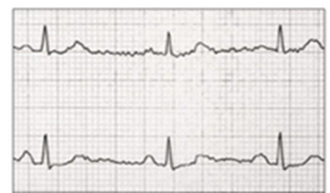
Fig.2. Application examples: electrocardiogram, weather forecast.

There are four time series properties quite accuratly describing its features:

• period — is a period with a constant length within the series and on the ends of which series has close values;
• seasonal — periodicity property (season=period);
• cycle — series characteristic changes due to global circumstances (for instance, economic cycles), there is no permanent period;
• trend — a tendency of time series values to increase or decrease.

Time series may contain anomalies. Anomaly is a deviation in a process standard behavior. Machine anomaly detection algorithms use process operation data (datasets). Depending on the subject area, a dataset may include various anomalies. There are several types of anomalies:

• point anomalies are characterized by behavior deviation in separate points;
• group anomalies are characterized by point group abnormal behavior, yet separately these points are not abnormal;
• contextual anomalies are characterized by connection to external data unrelated to series values (for example, negative outside temperatures during summer season).

Point anomalies are the easiest to detect: these are the points where process behavior differs a lot from other points. For example, a significant parameter value deviation is observed in a separate point.

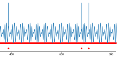
Fig.3. Several point anomalies.

Such values are called outliers. They have a significant impact on the statistical figures of the process, though outliers are easy to detect by setting a threshold for the observed value.

It is harder to detect an anomaly when the process behaves “normally” at every point, but joint values in different points have “strange” behavior. An example of such strange behavior is alternations in signal form, statistical figures (average value, mode, median, dispersion), intercorrelation emerging between two parameters, minor or short-term amplitude anomalous changes, etc. In this case, the challenge lies in detecting parameters’ anomalous behavior undetectable by standard statistical methods.

Fig.4. Group anomaly, frequency variation.

Anomalies detection is vital. In one case, we need to cleanse data to get a clear insight, in the other, anomalies should be thoroughly examined as they indicate that the observed system is close to emergency operation mode.

It is very complicated to detect anomalies in time series (unprecise anomaly detection, no labeling, unobvious correlation). Comprehensive state-of-the-art algorithms for detecting anomalies in time series have a high False Positive level.

Some anomalies can be detected manually (mainly point anomalies), if a good data visualization is provided. However, group anomalies are more difficult to detect, especially if there is a significant amount of data and analysis is required for information from several devices. “Anomalies in time” are also difficult to detect since a signal with normal parameters may appear at the “wrong time”. Therefore, for time series, it makes more sense to apply automation to anomalies detection methods.

Anomalies detection in real-life data poses another problem. It is usually unlabeled and, therefore, no initial strict anomaly definition and no rules for its detection exist. Under such circumstances, unsupervised learning methods, where models independently determine interconnections and distinctive patterns in data, are more appropriate.

Algorithms for anomalies detection in time series are often divided into three groups [3]:

• proximity-based methods are used for anomaly detection based on information about parameters proximity or fixed-length sequence parameters, suite for point anomaly and outlier detection but unable to detect changes in signal form;
• prediction-based methods build prediction model and compare their prediction with an original value, work best with time series with expressed periods, cycles or seasonality;
• reconstruction-based methods use reconstructed data pieces; therefore, they can detect both point and group anomalies, including changes in signal form.

Proximity-based methods are intended for detecting values significantly deviating from the behavior of all other points. The simplest example of this method implementation is threshold control.

The main goal of prediction-based methods is building a qualitative process model to simulate the signal and compare the obtained modeled values with the original ones (true). If the predicted and the true signals have close values, then the system behavior is considered “normal”; if the values in the model differ from the true values, the system behavior will be declared anomalous at this segment.

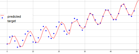
Fig.5. Time series modeling.

SARIMA [4] and recurrent neural networks [5] are the most popular methods for time series modeling.

An original approach is implemented in reconstruction-based models: at first, the model is trained to encode and decode signals from an available selection, while the coded signal has a significantly smaller dimension than the original. Therefore, it is required to “compress” information. An example of such compression for 32×32 pixels pictures to 32 number matrix is represented below.

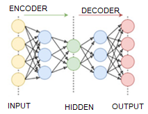
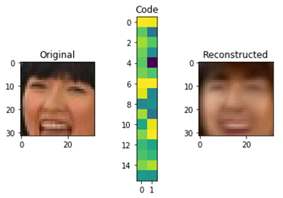
Fig.6. Autoencoder operation scheme.

After the model training is complete, segments of the examined time series are used as input signals. If encoding-decoding is successful, the process behavior will be considered “normal”; otherwise, its behavior will be deemed anomalous.

One of the recently developed reconstruction-based methods is TadGAN [3] which has achieved impressive results on anomalies detection. It was developed by MIT researchers at the end of 2020. TadGAN method architecture contains an autoencoder and a generative adversarial network elements.

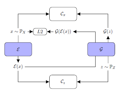
Fig.7. TadGAN architecture (from article [3])

Ɛ acts as an encoder mapping x time series sequences into z latent space vectors, and G is a decoder, reconstructing time series sequences from a latent representation z. Cx is a critic, evaluating G(Ɛ(х)) reconstruction quality, and Cz is a critic evaluating z = Ɛ(х) latent representation similarity to white noise. Besides, “similarity” control of the original and the reconstructed samples is applied using L2-measure based on “Cycle consistency loss” ideology (ensures common similarity of generated samples with the original samples in GAN) [6]. The resulting target function is a sum of all metrics intended to evaluate the quality of Cx, Cz critics operation, and the original and the reconstructed signals similarity measures.

Various standard high level API packages (e.g. TensorFlow or PyTorch) may be used to create and train neural networks. In the repository [7], you can find an implementation example of an architecture similar to TadGAN, where the TensorFlow package is used for weights training. During model training five metrics were optimized:

• aeLoss — mean square deviation between the original and the reconstructed time series in other words a discrepancy between x and G(Ɛ(х)),
• cxLoss — the Cx critic binary cross entropy, determining difference between the original time series segment and the artificially generated one,
• cx_g_Loss — binary cross-entropy, a G(Ɛ(х)) generator error, characterizing its incapability to “fool” the Cx critic,
• czLoss — the Cz critic binary cross-entropy, determining the difference between latent vector generated by the Ɛ encoder and white noise, ensures Ɛ(х) latent vector similarity with a random vector preventing the model to “learn” separate patterns in the original data,
• cz_g_Loss — binary cross-entropy, a Ɛ(х) generator error, characterizing its incapability to create latent vectors similar to random ones and thereby “fool” the Cz critic.

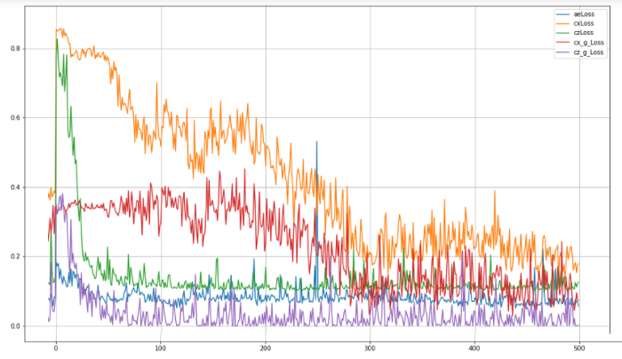
Fig.8. TadGAN model training quality for 500 epochs.

After the model training is complete, reconstruction of separate segments belonging to explored time series is executed; original and reconstructed series are to be compared by one of the following methods:

• point by point comparison;
• curve areas comparison in a field around each sample (width is a hyperparameter);
• Dynamic Time Warping [9].

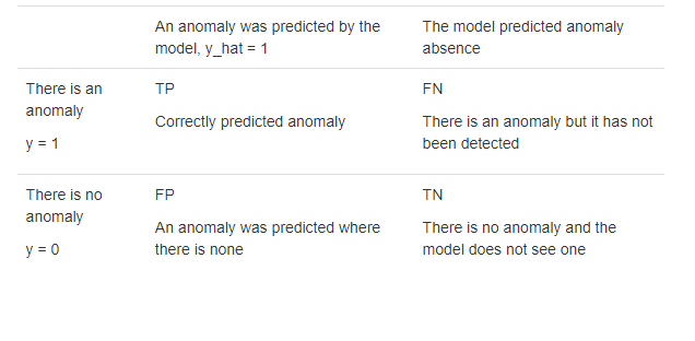
Binary classification problem quality is evaluated through F1-metric: “positive” (zero hypothesis) — there is an anomaly; “negative” (alternative hypothesis) — there is no anomaly.

To demonstrate how the method works, we will use synthetic (artificially created) series without anomalies. This series is a sum of two sinusoids which values vary in the range from -1 to 1.

The series curve:

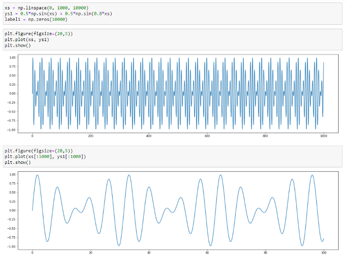
Fig.9. Synthetic series graph.

The series reconstructed by TadGAN for a various number of stages (4 and 80) will be as follows:

Fig.10. Series modeling by TadGAN for a different number of epochs (4 epochs — red, 80 epochs — green).

We can see that the model has learnt to predict main patterns in data. Let’s try addiing various anomalies in data and then detecting them by the TadGAN model. At first, we are going to add a few point anomalies.

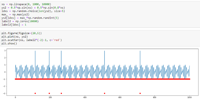
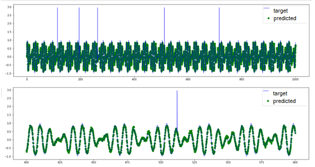
Fig.11. Point anomaly detection by TadGAN

Based on the original and the predicted signal curves, we can see that the model cannot reconstruct anomalous value “peaks”; however, it can detect point anomalies with high accuracy. In this case, it is difficult to see what benefit we gain using such a sophisticated model as TadGAN because similar anomalies can be detected by the threshold exceeding evaluation.

And now, let’s turn to a signal with another anomaly type: periodic signal with anomalous frequency variations. There is no threshold exceeding here. All series elements have “normal” values from the perspective of amplitude, and the anomaly is detected only in the group behavior of several points. TadGAN is also incapable to reconstruct a signal (as you can see in the picture) and cannot be used as evidence of a group anomaly.

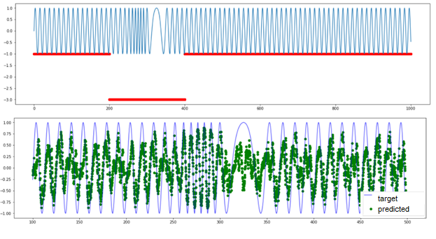
Fig.12. Results TadGAN operation on a dataset with anomalous frequency variations.

These two examples illustrate how the method works. You can try creating your own datasets and check the model capabilities in various situations.

More complicated dataset examples were published by the TadGAN developers in their article. There is also a link to another MIT specialist development — the Orion library, capable of detecting rare anomalies in time series applying the unsupervised machine learning approach.

As a conclusion, there is a lot of various comprehensive anomaly detection methods implementing signal reconstruction (reconstruction-based); for instance, arxiv.org contains dozens of articles describing various modifications to the approach, implementing autoencoders and generative adversarial networks. It is highly advisable to choose a specific model for each problem considering its requirements and subject area.

The technology described in this article has practical application in CL Thymus, CyberLympha’s AI/ML-based software, designed to protect OT networks and Industrial Control Systems that operate data exchange protocols based on unknown or proprietary protocols with no specifications available to the public. More info about CyberLympha and its products is available on the company website.

References

1. “What is a data analytics?” (ru), https://www.intel.ru/content/www/ru/ru/analytics/what-is-data-analytics.html
2. Dombrovsky. “Econometrics” (ru). http://sun.tsu.ru/mminfo/2016/Dombrovski/start.htm
3. “TadGAN: Time Series Anomaly Detection Using Generative Adversarial Networks”, https://arxiv.org/abs/2009.07769
4. “An Introductory Study on Time Series Modeling and Forecasting”, описание SARIMA https://arxiv.org/ftp/arxiv/papers/1302/1302.6613.pdf
5. Fundamentals of RNN, https://arxiv.org/abs/1808.03314
6. Cycle Consistency Loss, https://paperswithcode.com/method/cycle-consistency-loss
7. https://github.com/CyberLympha/TadGAN
8. Orion, a library for anomaly detection, https://github.com/signals-dev/Orion
9. Dynamic Time Warping algorythm description, https://towardsdatascience.com/dynamic-time-warping-3933f25fcdd
10. https://medium.com/mit-data-to-ai-lab/time-series-anomaly-detection-in-the-era-of-deep-learning-dccb2fb58fd
11. https://medium.com/mit-data-to-ai-lab/time-series-anomaly-detection-in-the-era-of-deep-learning-f0237902224a